R

R is a language and environment for statistical computing and graphics. It is a GNU project which is similar to the S language and environment, developed at Bell Laboratories.

R provides a wide variety of statistical such as linear and nonlinear modelling, classical statistical tests, time-series analysis, classification, clustering and graphical techniques, etc… and is highly extensible.

Cleaning with R

The scenario

Working as a data analyst working for a hotel booking company, the main task is to clean a .csv file that was created after querying a database to combine two different tables from different hotels.

In order to learn more about this data, I am going to use functions to preview the data’s structure, including its columns and rows. In addition, I am going to use basic cleaning functions to prepare this data for future analysis.

Step 0: Download the data

Click on the file below to download the data set:

• hotel_bookings.csv

Step 1: Load packages

In order to start cleaning the data, I first install and load the required packages, that is tidyverse, skimr, and janitor.

install.packages("tidyverse")
install.packages("skimr")
install.packages("janitor")

Once a package is installed, it has to be loaded by running the library() function, with the package name inside the parentheses:

library(tidyverse)
library(skimr)
library(janitor)

Step 2: Import data

The data is currently an external .csv file. In order to view and clean it in R, I need to import it. The tidyverse library readr package has a number of functions for “reading in” or importing data, including .csv files.

I use the read_csv() function to import data from a .csv file in the project folder called “hotel_bookings.csv” and save it as a data frame called bookings_df:

bookings_df <- read_csv("hotel_bookings.csv")

Step 3: Getting to know your data

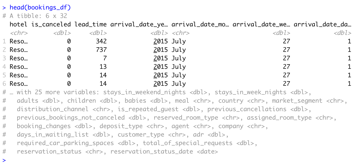
Before you start cleaning the data, it is important to take some time to explore it. There are several functions to preview the data, including the head() function in the code chunk below:

head(bookings_df)

Data can also be summarized or previewed with the str() and glimpse() functions to get a better understanding of the data by running the code chunks below:

str(bookings_df)

glimpse(bookings_df)

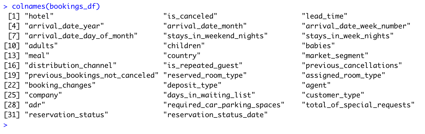
Also, colnames() to check the names of the columns in your data set is useful:

colnames(bookings_df)

Some packages contain more advanced functions for summarizing and exploring your data. One example is the skimr package, which has a number of functions for this purpose. For example, the skim_without_charts() function provides a detailed summary of the data:

skim_without_charts(bookings_df)

Step 4: Cleaning the data

Based on the functions used so far it is possible to describe the data in a brief to the stakeholder. Now, let’s say we are primarily interested in the following variables: ‘hotel’, ‘is_canceled’, and ‘lead_time’.

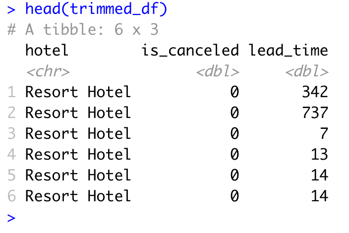
I then create a new data frame with just those columns, calling it trimmed_df by adding the variable names to this code chunk:

trimmed_df <- bookings_df %>% 
  select(hotel, is_canceled, lead_time)

head(trimmed_df)

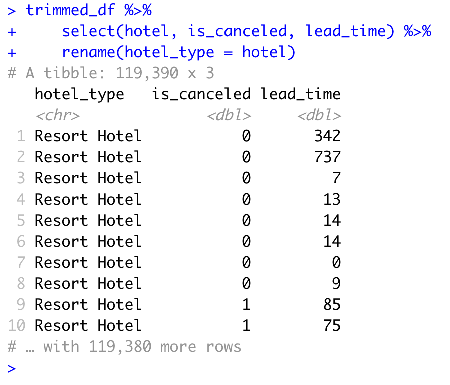
Since some of the column names aren’t very intuitive, will want to rename them to make them easier to understand. So I create the same exact data frame as above, but rename the variable ‘hotel’ to be named ‘hotel_type’ to be crystal clear on what the data is about…

trimmed_df %>% 
  select(hotel, is_canceled, lead_time) %>% 
  rename(hotel_type = hotel)

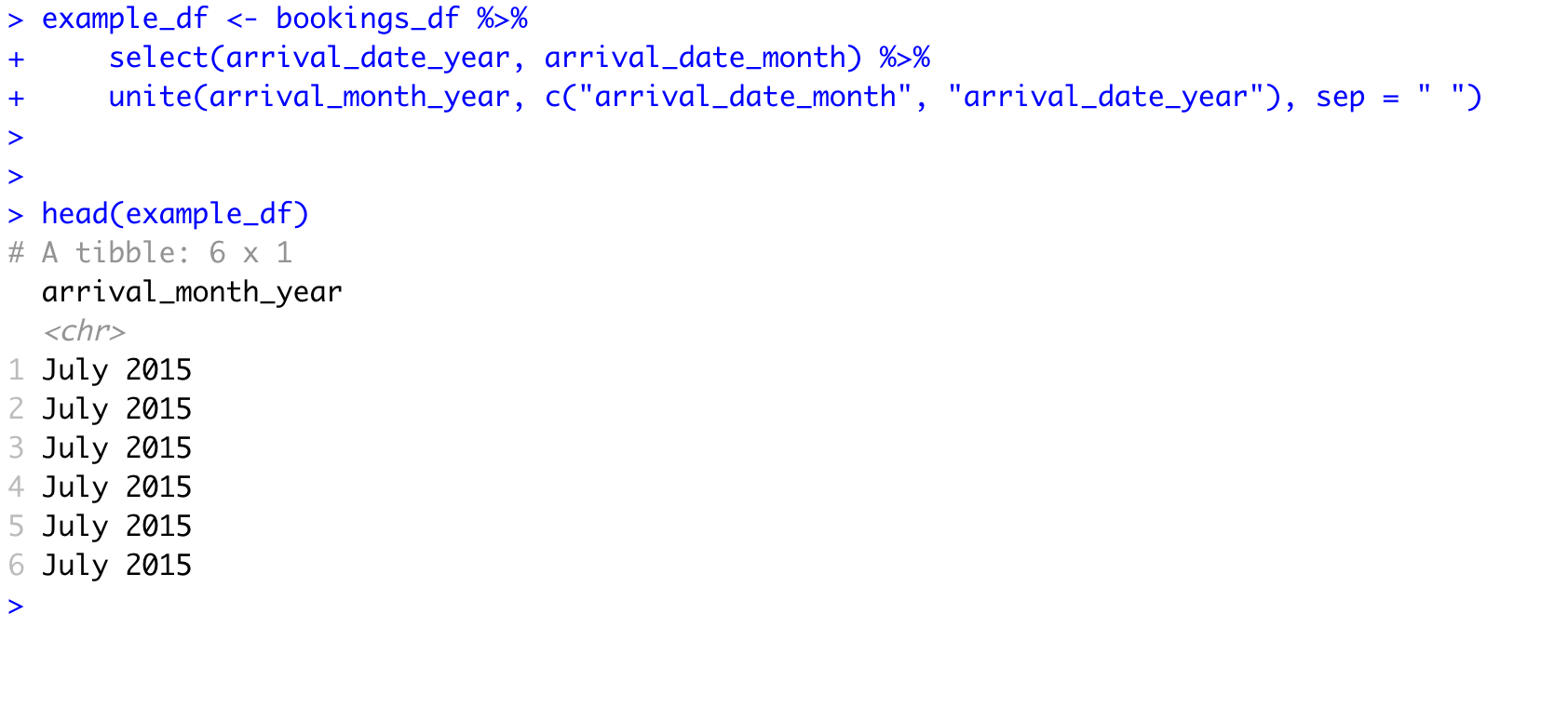
Another common task is to either split or combine data in different columns. In this example, it is possible to combine the arrival month and year into one column using the unite() function:

example_df <- bookings_df %>%
  select(arrival_date_year, arrival_date_month) %>% 
  unite(arrival_month_year, c("arrival_date_month", "arrival_date_year"), sep = " ")

Step 5: Another way of doing things

It is possible to also use the mutate() function to make changes to the columns. Let’s say I wanted to create a new column that summed up all the adults, children, and babies on a reservation for the total number of people. Modify the code chunk below to create that new column:

example_df <- bookings_df %>%
  mutate(guests = adults + children + babies)

Great. Now it’s time to calculate some summary statistics!

TO calculate the total number of canceled bookings and the average lead time for booking, I first make a column called ‘number_canceled’ to represent the total number of canceled bookings. Then, another column called ‘average_lead_time’ to represent the average lead time.

Use the summarize() function to do this in the code chunk below:

example_df <- bookings_df %>%
  summarize(number_canceled = sum(is_canceled),
            average_lead_time = mean(lead_time))

head(example_df)